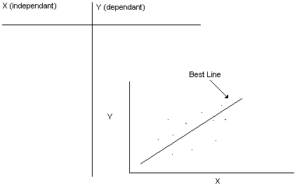
Mean = (å xi)/n
Variance d = (å xi2)/n - (mean)2
Covariance m xy = (å xi yi)/n - (x)(y)
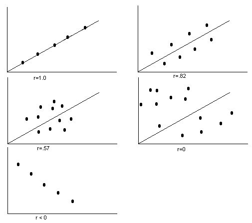
Correlation = r
Regression; y = mx + b
CIS 375 SOFTWARE ENGINEERING
University Of Michigan-Dearborn
Dr. Bruce Maxim, Instructor
Regression And Correlation.

Mean = (å xi)/n
Variance d = (å xi2)/n - (mean)2
Covariance m xy = (å xi yi)/n - (x)(y)
Correlation = r
Regression; y = mx + b
|
X |
Y |
X^2 |
X*Y |
Y^2 |
|
1 |
1 |
1 |
1 |
1 |
|
3 |
2 |
9 |
6 |
4 |
|
4 |
4 |
16 |
16 |
16 |
|
6 |
4 |
36 |
24 |
16 |
|
8 |
5 |
64 |
40 |
25 |
|
9 |
7 |
81 |
63 |
49 |
|
11 |
8 |
121 |
88 |
64 |
|
14 |
9 |
190 |
126 |
81 |
|
S= 56 |
40 |
524 |
364 |
256 |
Regression Models
1. Linear Model
E = Co + S Cix
{Effort in Person Months} {Intercept} {Regression Coefficient}
2. Static Non-Linear Model
n
E = Co + S Cix xi2i
i=1
Often rewritten using size of code as a factor
E = a + b Sc m (x) n
{where a, b & c are constants, S = size, m = multiplier, and x = S Cix xi2i }
i=1
COCOMO Model
COnstructive COst MOdel
Contains 3 levels
1. Basic: Computes software development effort (and cost) as a function of program size, expressed in estimated lines of code.
2. Intermediate: Computes software development effort as a function of program size and a set of "cost drivers" that include subjective assessments of product, hardware, personnel, and project attributes.
3. Detailed: Includes all characteristics of the intermediate version with an assessment of the cost driver’s impact on each step (analysis, design, ect.) of the software engineering process.
Model: E = a Sb m(x)
|
BASIC |
INTERMEDIATE |
|||
|
MODE |
a |
b |
a |
b |
|
Organic |
2.4 |
1.05 |
3.2 |
1.05 |
|
Semidetached |
3.0 |
1.12 |
3.0 |
1.12 |
|
Embedded |
3.6 |
1.20 |
2.8 |
1.20 |
in the basic COCOMO model x=1
in the intermediate model a questionnaire is used
|
Product Attributes |
Computer Attributes |
||
|
RELY |
Reliability |
TIME |
Execution Time |
|
DATA |
Size of database |
STOR |
Amount of Storage |
|
CPLX |
Complexity of System |
VIRT |
Virtual Volatility |
|
* |
* |
TURN |
Response Time |
|
Personnel |
Project |
||
|
ACAP |
Analyst Capabilities |
MODP |
Modern Practices |
|
AEXP |
Analyst Experience |
TOOL |
Software Tools |
|
PCAP |
Programmer Capabilities |
SCED |
Development Schedule |
|
PEXP |
Programmer Experience |
* |
* |
|
VEXP |
Machine Experience |
* |
* |
|
LEXP |
Language Experience |
* |
* |
Dynamic Estimation Models:
(Rayliegh curve -> skewed, median & mean offset from one another).
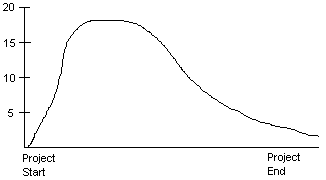
Based on:
E = y(t
{t represents optimal time} {K represents the area under the Rayliegh curve}.
D = K / t
2;{difficulty measure based on t
2 and K}.P = C2D-2/3;
{productivity measure}.
Ss = c K-1/5 t 4/3;
{ lines of code measure} {c represents the technology factor from survey}.
Staff (t) = sech2 [(a t + c)/2].
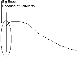
(less sensitive to compression)
Ss = Cte T K 1/2
{ Cte represents technology constraint with environmental adjustment}.
E = E1 (S) + E2 (m);
{E represents total effort}.
{E1(S) represents the effort of one or people working independently
E1(S) = a + bs ,where a & b are empirically derived constants}.
{E2(m) represents the effort required to coordinate the development process
E2(m) = cm2 where m is the average number of team members}.
Make-Buy-Decision:
Decision Steps:
Now you’re in a good position to evaluate.
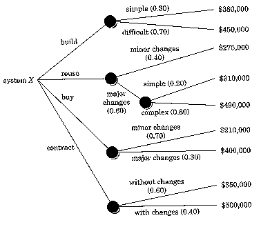
One way: build a decision tree.
