
CIS 375 SOFTWARE ENGINEERING
University Of Michigan-Dearborn
Dr. Bruce Maxim, Instructor
ERPP:
Evolutionary rapid prototyping process.
(Write less throwaway code than in spiral model)
Start with Product Plan:

Risks Using ERPP:
Requirements Analysis For ERPP:
Design:
(Always has one process, even in ERRP model)
Implementation & Testing:
Final Spin Cycle:
1) Prototype -> spaghetti code.
Requirements Specification Methods:
(Hierarchy Input - Output Chart)
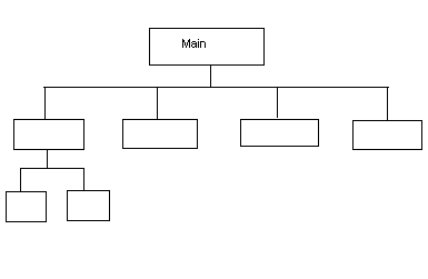
Strengths Weaknesses
- Shows function - No mechanism for
relationship. Non-functional requirements.
- No checking mechanism.
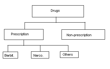
How is it different from object hierarchy:
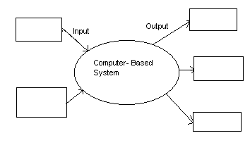
{square} = producer or consumer of information.
{circle} = software client capable of transforming information.
{arrow} = data item.
{thing} = database.
Key: this is data flow.
PSPEC - process specification.
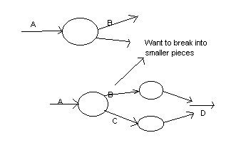
Control flow diagram.
CSPEC - control specification.
Data object tables are determined.
Object = record.
Attribute = fields.
Normalization Rules:
E-R Diagram:
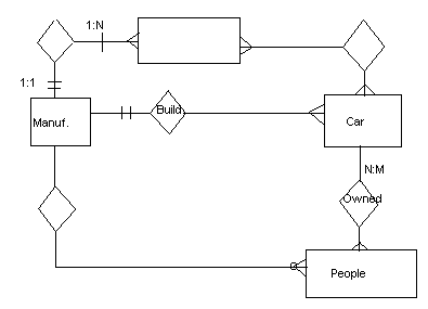 (Entity relationship)
{squares} = data object.
{diamonds} = relationship between objects.
|
Rules |
|||
|
Condition |
1 |
2 |
|
|
Rules |
|||
|
Actions |
1 |
2 |
|
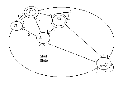 Transition functions - ò
: ò
* å
®
ò
.
Transition functions - ò
: ò
* å
®
ò
.(Like decision table)
|
Mode |
Event1 |
Event2 |
Event3 |
Event4 |
|
Presentation Graphics |
Action1 |
Action8 |
O |
X |
|
Architecture Drawing |
X |
A2 then A3 |
A5 & A6 |
O |
|
Programming |
O |
A4 |
A1, A2 & A3 |
A7 |
O = no action / no state change.
X = no action defined.
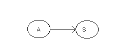 Sequential processes.
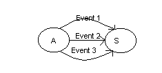 f(state A, event) -> state S.
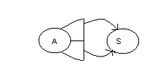 f(state A, event1, event2, event3) -> state S.
f(state A, event1, event2, event3) -> (state S1, state S2).
Structured analysis activity diagram:
(Activity Network)
Control
¯
Inputs® ¬ Output
Mechanism
Structured analysis data diagram:
(Data Network)
Control
¯
Generating Activity® ¬ Resulting Activity
Storage Devices
Design techniques:
Explains how to interpret results of SA (control issues).
(Database way of attacking things)
(a.k.a. data dictionary)
Procedural Design: (cont.)
{figure 53}
{figure 54}
Perspective of the system as data transforms.